Project Methods

Current UMORF 3D Acquisition Methods (as of July 2017)

Our current 3D acquisition workflow was initially developed in 2014 by collection manager Adam Rountrey and UM undergraduate David Vander Weele.  UM undergraduate Briar Scott has continued to improve software and processes over the past year, and UM graduate student James Saulsbury recently created a portable system based on the original workflow.  The general pattern is to use a turntable and camera to capture around 150 photographs in a series of six or more “rings” around the object, and then use photogrammetry software to produce a 3D model.
General Features
Object size: ~5mm to ~1000mm for our standard station (larger possible).
Resolution: Typically, features larger than about 100 microns are resolvable
Model Size: Most models have between 5 and 20 million faces.  Our largest model consists of 1.1 billion faces.  Models are reduced to 2 million faces or less for web viewing on UMORF.
Color: All models are produced with color information.  We use vertex color rather than UV texture mapping to avoid representing color information that is beyond the geometric resolution of the model
Time: Semi-automated photography takes around 20 minutes per object.  Reconstruction for typical objects takes less than one hour compute time.

Light box and camera

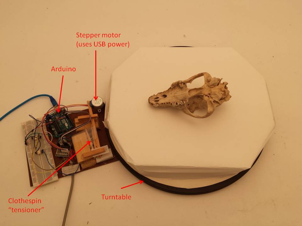
Turntable with Arduino and stepper motor

Equipment
Camera: Nikon D810 camera with 60mm macro lens.
Light Box: 48” custom three-sided enclosure made from corrugated polypropylene and paper.  The top and camera side are covered only with white disposable plastic tablecloth (performs better than fabric).  Two 500W halogen lights shine through the tablecloth on the top of the enclosure (these have now been replaced by four LED panels).  Very diffuse lighting is essential.
Semi-automatic turntable: A plastic turntable designed for large televisions is driven by a small stepper motor connected to an Arduino.  Software written for the Arduino rotates the turntable, stopping every X degrees and triggering the shutter on the camera.  Photography can also be done manually.

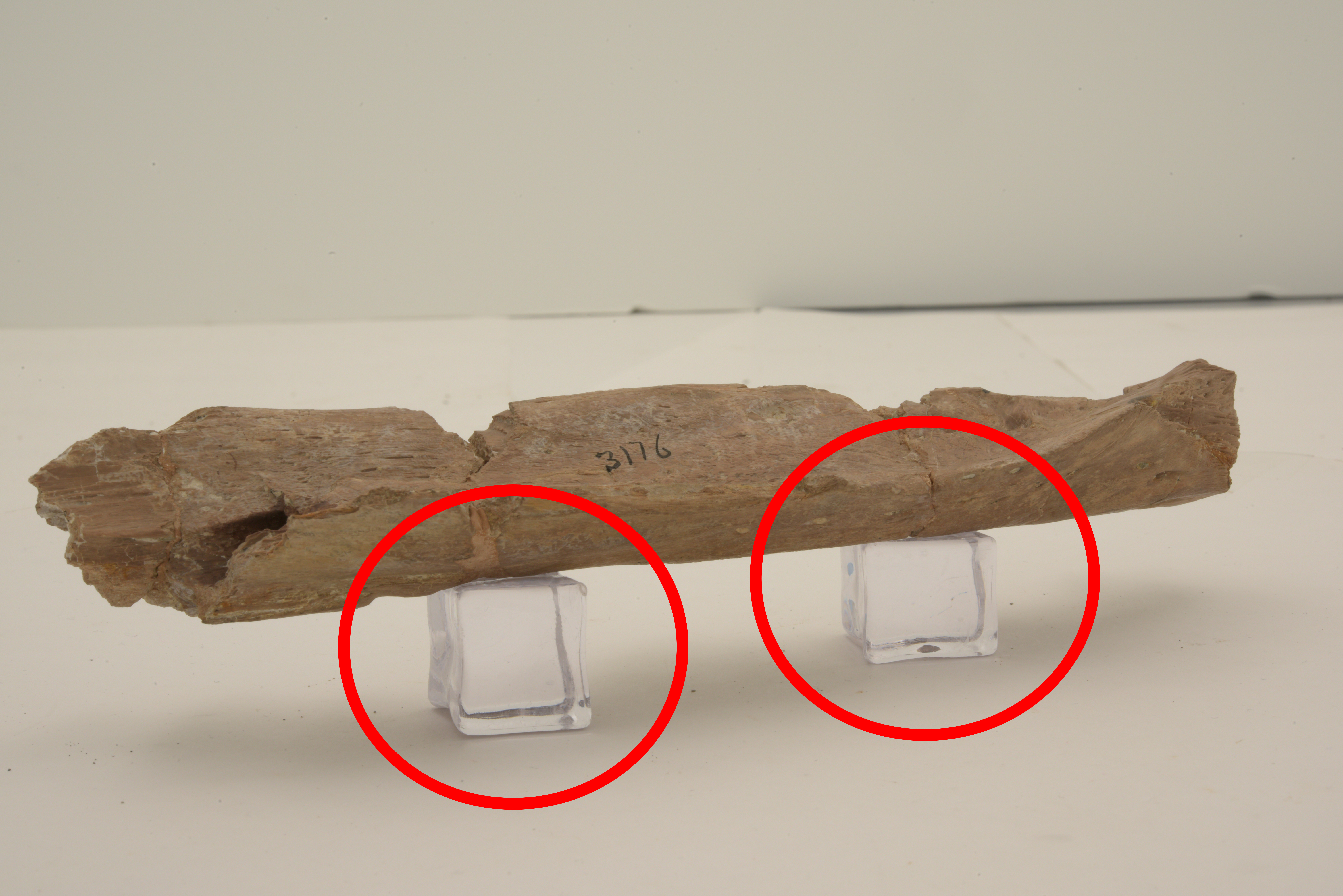
Acrylic Ice Cube Support

“Ice” Cubes: Specimens are generally placed on top of clear acrylic “ice cubes” on the turntable.  These cubes have wavy sides and bend light in ways that result in a lack of stable features in images.  In other words, they are invisible to photogrammetry algorithms!  Placing them under specimens prevents the turntable background from “attaching” to the object model, and it allows more light to reach the underside of the specimen during photography.

Workstation: HP Z840 1125W workstation with 2 Xeon E5-2623v3 3.0 Ghz 4 Core CPUs, 128 GB RAM, Nvidia Titan X GPU.  Reconstruction can be accomplished on lower performance workstations, but a good GPU (~Nvidia GTX 970 or better) is essential.

Photogrammetry software

Process

1. Place the object at center of turntable with side 1 up.
2. Position the camera such that the angle between the view direction and the plane of the turntable is about 60 degrees. It is simplest if the entire object will be in every frame as the turntable rotates, but this is not necessary.  Including smaller parts of the object in each frame will require more photos to get full coverage.
3. Set the f-stop to f/32 (despite diffraction, we found this aperture setting to produce the best results in our system). Do not use auto-white balance, and make sure the ISO is set as low as possible (64 in our case).
4. Focus the camera manually at the center of the object.
5. Initiate a set of ~25 photos for one rotation of the turntable (or manually take around 25 photos in a “ring” around the object).
6. Reposition the camera at a 45-degree angle and repeat steps 4 and 5.
7. Reposition the camera at a 10-degree angle and repeat steps 4 and 5.
8. Flip the object 180 degrees so that side 2 is facing up.
9. Repeat steps 4 and 5.
10. Reposition the camera at a 45-degree angle and repeat steps 3 and 4.
11. Reposition the camera at a 60-degree angle and repeat steps 3 and 4.
12. Process the photos in Reality Capture to produce a model.

Note: We generally scale models after they have been produced in Reality Capture.  The models are opened in MeshLab, and two points on the model that can also be found on the object are identified.  These should be very small features allowing precise measurement.  Measure the distance between the features in MeshLab and the distance between the features on the object (we use calipers) and calculate the scaling factor required.  Use your scaling factor with MeshLab’s scale function.  We measure two additional features on the scaled model to confirm that the scaling was accurate.

Project Methods (for most models made before 2014)

Most of our 3D models start with a surface model of a specimen. Some of these were created with a Microscribe 3DLX point digitizer. More recently, many of our models have been generated with a Creaform HandyScan laser-scanning digitizer. Models from the invertebrate Type and Figured Collection were produced using a “visual hull” approach, implemented in the commercial software 3DSOM Pro. Still others were derived from photogrammetry (using PhotoModeler, Autodesk 123D Catch, or VisualSFM + CMPMVS) or from x-ray computed tomography scans.

Texture-mapping to give models a photorealistic appearance has been done mostly with 3DSOM Pro. In this procedure, 2D images of a specimen are extracted from their background and then projected onto the surface of the model, aligning them to topographic features of the model. Multiple images from different positions around the form blend to approximate the local color and texture of the original specimen. Onscreen exploration of these texture-mapped models offers a close approximation to the experience of handling the original specimens yourself.

VisualSFM
Wu, C. (2013).  Towards Linear-time Incremental Structure from Motion. 3DV.
Wu, C. (2007). SiftGPU: A GPU implementation of Scale Invariant Feature Transform (SIFT). http://cs.unc.edu/~ccwu/siftgpu.
Wu, C., Agarwal, S., Curless, B., Seitz, S.M. (2011). Multicore Bundle Adjustment. CVPR.

CMPMVS
Jancosek, M., Pajdla, T. (2011). Multi-View Reconstruction Preserving Weakly-Supported Surfaces. 2011 – IEEE Conference on Computer Vision and Pattern Recognition.